Jet Fuel Demand

Data

For a start, we have limited the modelling scope to US jet fuel consumption, and have incorporated publicly available monthly data from the U.S. Energy Information Administration (EIA) from 2004 to 2016 (2017 to 2019 has been reserved for model testing). And where necessary, we have converted the monthly data to quarterly on a cumulative basis to better correspond with commodity supply and demand data.

Visualizing and Decomposing the Time Series Data

Time series data is by nature temporal and arguably challenging to construct forecasting models for. Visual observations of the time series data already display signs of non-stationarity across trend, seasonality and variance.

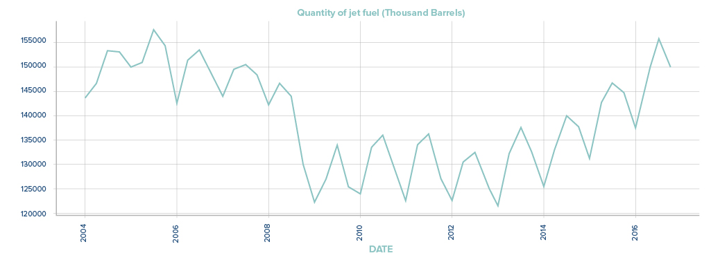
Here is a first look at the data for the period 2004-2016 (y-axis: Jet Fuel ‘000 bbls, x-axis: Quarters for the period).

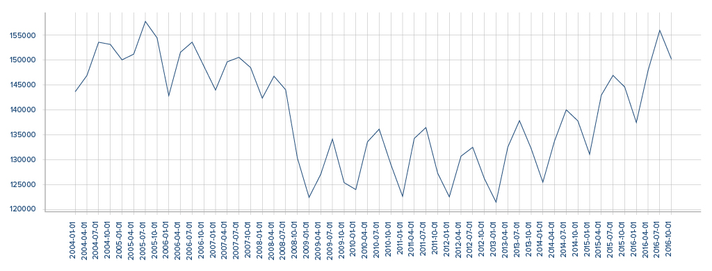
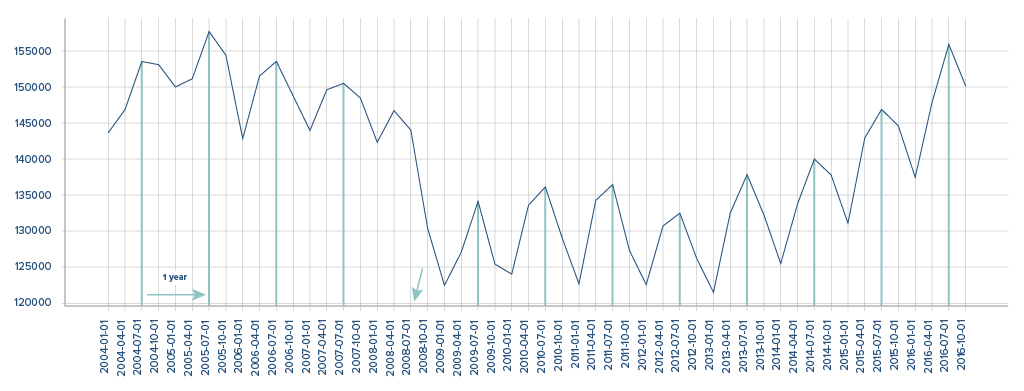
The first history lesson would be that the demand trough over the 2004-2016 period corresponds nicely with the Great Financial Crisis of 2008-2009, with sustained recovery kicking in only years later in 2013. The other observation corresponds with the known seasonal nature of most commodities including jet fuel – notably accentuated by (Northern Hemisphere) summer peaks and winter troughs. Ignoring the lags in data collection, the strong seasonal pattern in jet fuel consumption in most years with the exception of 2008 (red arrow) is unmistakable. Plausible, given the seasonal nature of vacation travel and the severe impact of the financial crisis on incomes in 2008 and thereafter.

Breaking down the jet fuel time series data into the components, the observations become more pronounced.

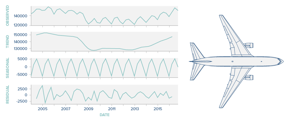
Data Stationarity

Trend stationarity is debatable given the observations of a trough, but perhaps less debatable would be the strong seasonality pattern exhibited by the data. Achieving stationarity looks to be complex as we seek to stabilise the statistical properties (mean, variance) of the time series data for a meaningful forecasting model to be built.

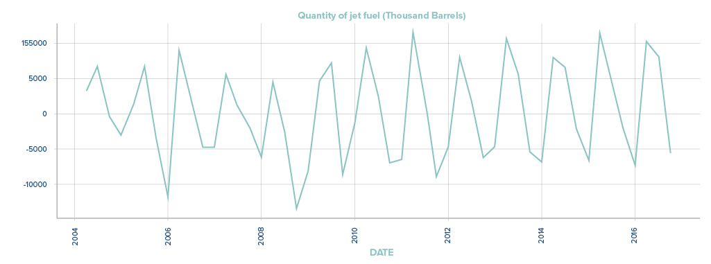
With first order differencing, the spread of the data reduces significantly and the Augmented Dicky-Fuller (ADF) test yields a p-value of 0.626. Statistically, a p-value of less than 0.05 would indicate data stationarity. But since the p-value is greater than 0.05, this necessitates differencing the data by a second time.

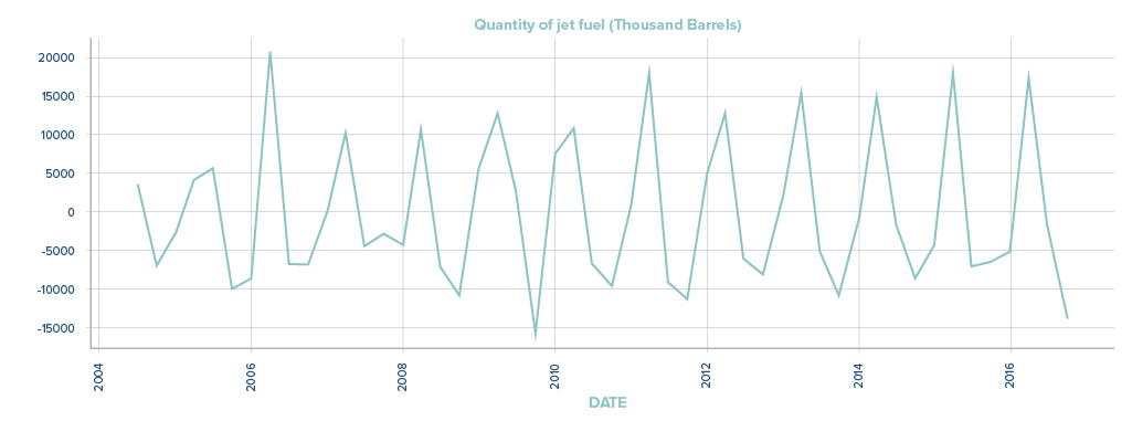
After differencing the data a second time, we reduce the spread of the data even further. Now, the ADF test yields a p-value of 0, which is < 0.05 and indicates that the data can be applied for modelling. Note that in the graph below, that the forecast results have been inverted to allow interpretation of the two orders of differencing applied earlier to the data.

Goals of Predictive Modelling

Mathematics is the language of nature – or divinity for some. Sidestepping misguided attempts in the search for any holy grail, in predictive modelling we focus on generating forecasts for possible future unknown outcomes while minimising prediction error. In this project, we’ve trained the model on 2004-2016 data, with a view to testing the predictive capabilities in the 2017 to 2019 period.

Conditions for forecasting

We have assumed that history is doomed to repeat itself in some manner or other, in order to derive reliable forecasts. And for this reason, we have omitted COVID-stricken periods (2020-2021), which more likely resemble stress test scenarios. For sanity reasons, we have left modelling to account for black swans or extreme outcomes like COVID as a brave endeavour for our next project.

Forecasting Approaches

And for simplicity, we have sought to arrive at the best performing model using the Mean Absolute Percentage Error (MAPE) as a key metric for measuring predictive accuracy and reliability. In this project, we explore the intuition behind two models: Autoregression and Facebook Prophet.

Autoregression

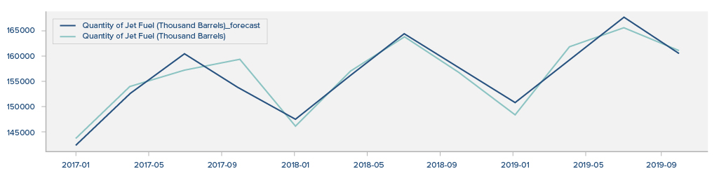
Autoregressive models forecast a series based on preceding time lags – we use past values of jet fuel consumption data to predict future values, iteratively testing different lag periods and the corresponding predictions.

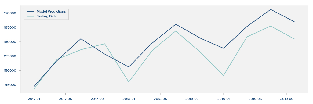
While there are noticeable points with large margins of error (2019-01), the MAPE for this autoregressive model is 2.57%.

Prophet

Prophet is a time series forecasting tool developed by Facebook to accommodate a wide range of business use cases. It uses the decompositions we discussed earlier with three main components: trend, seasonality, and holidays. Instead of directly relying on past values for forecasting, the forecasting problem is framed as a curve-fitting exercise by looking at the data as a scatterplot. This is starkly different from the autoregressive model in that it does not explicitly account for dependence on time. These qualities make Prophet suitable for data with strong seasonal effects.

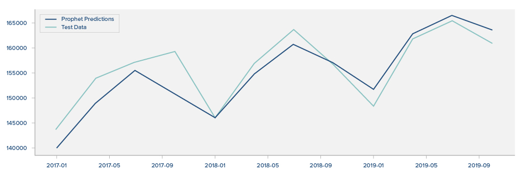
Visually, the Prophet seems to outperform the autoregressive model, and proves so with a MAPE of 1.7%.

Adding More to the Model: Vector Autoregression

We conjecture that univariate models may be insufficiently robust to deal with the multi-faceted nature of jet fuel consumption. In exploring multivariate techniques such as Vector Autoregression (VAR), we included other variables such as the load factor (% of airplane’s occupied capacity) and personal income per capita as other predictors for the model. While not significantly so, the VAR model seems to outperform our previous two with a MAPE of 1.2%.

Forecasting into the Future

With a selection of models, we will now reintegrate the testing data (2017-2019) together with the training data (2004-2016). We make no forecasts on extreme distortionary events, but will utilise the models in estimating the impending consumption recovery from COVID based on some of the data variables used. A resumption of pre-COVID consumption behavioural patterns post-COVID, will have significant impact on air and land based travel, albeit with some subtle data differences.

---

Disclaimer

Please refer to our terms and conditions for the full disclaimer for Stoic Capital Pte Limited (“Stoic Capital”). No part of this article can be reproduced, redistributed, in any form, whether in whole or part for any purpose without the prior consent of Stoic Capital. The views expressed here reflect the personal views of the staff of Stoic Capital. This article is published strictly for general information and consumption only and not to be regarded as research nor does it constitute an offer, an invitation to offer, a solicitation or a recommendation, financial and/or investment advice of any nature whatsoever by Stoic Capital. Whilst Stoic Capital has taken care to ensure that the information contained therein is complete and accurate, this article is provided on an “as is” basis and using Stoic Capital’s own rates, calculations and methodology. No warranty is given and no liability is accepted by Stoic Capital, its directors and officers for any loss arising directly or indirectly as a result of your acting or relying on any information in this update. This publication is not directed to, or intended for distribution to or use by, any person or entity who is a citizen or resident of or located in any locality, state, country or other jurisdiction where such distribution, publication, availability or use would be contrary to law or regulation.